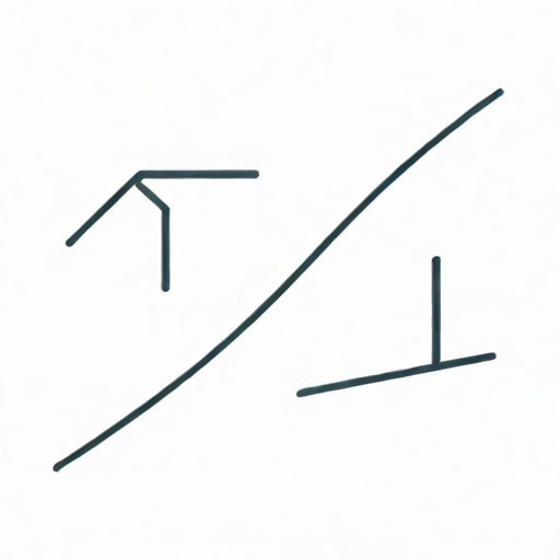
In mathematics, particularly in algebra and calculus, the concepts of oblique asymptotes and slant asymptotes are essential for understanding the behavior of rational functions as the input values become extremely large or small. Both terms are often used interchangeably, but their usage and context can sometimes differ, leading to confusion among students and practitioners. An asymptote is a line that a graph approaches but never touches or crosses in certain cases, and it helps describe the long-term behavior of functions. Oblique asymptotes, also known as slant asymptotes, appear when the degree of the numerator of a rational function is exactly one more than the degree of the denominator. Understanding these asymptotes is critical for graphing, analyzing, and interpreting rational functions, which have applications in physics, engineering, economics, and other fields where modeling continuous change is essential.
Definition of Oblique Asymptotes
An oblique asymptote is a straight line that a graph of a function approaches as the independent variable (usually x) tends to positive or negative infinity, but the line is not horizontal or vertical. Unlike horizontal asymptotes, which indicate that a function levels off to a constant value, oblique asymptotes show that the function grows without bound but in a linear fashion relative to the line. Oblique asymptotes are most commonly encountered in rational functions where the degree of the numerator is exactly one greater than the degree of the denominator.
Characteristics of Oblique Asymptotes
- The line has the general form y = mx + b, where m is the slope and b is the y-intercept.
- It occurs in rational functions when the degree of the numerator is one more than the degree of the denominator.
- The function approaches this line as x approaches positive or negative infinity.
- It provides a linear approximation of the function at extreme values of x.
Mathematically, to find the oblique asymptote of a function f(x) = P(x)/Q(x), one performs polynomial long division if the degree of P(x) is exactly one more than Q(x). The quotient, excluding the remainder, represents the equation of the oblique asymptote. This line indicates how the function behaves for very large or very small input values, which is critical for understanding trends in applied contexts such as population growth or financial modeling.
Understanding Slant Asymptotes
Slant asymptotes, often called oblique asymptotes, describe the same concept from a slightly different perspective. The term slant emphasizes the non-horizontal and non-vertical nature of the asymptote, focusing on the angle at which the function approaches the line. Essentially, a slant asymptote is a line that the function approximates at extreme x-values, and it appears as a slanted line on the graph. In practice, slant and oblique are synonymous, and the choice of term is largely based on regional or educational preferences. For students, understanding that slant asymptotes indicate a linear trend in the growth or decay of a function can simplify graphing and interpretation.
How to Determine a Slant Asymptote
The process of finding a slant asymptote mirrors that of an oblique asymptote
- Ensure the function is a rational function where the degree of the numerator is exactly one greater than the degree of the denominator.
- Use polynomial long division to divide the numerator by the denominator.
- Ignore the remainder, as it becomes insignificant for large x-values.
- The quotient represents the slant asymptote equation, typically in the form y = mx + b.
For example, consider the function f(x) = (2x^2 + 3x + 1)/(x + 1). The numerator has degree 2, and the denominator has degree 1, so a slant asymptote exists. Performing long division, the quotient is 2x + 1, which represents the slant asymptote. As x tends to infinity or negative infinity, the function f(x) approaches the line y = 2x + 1, illustrating its long-term linear behavior.
Graphical Interpretation
Graphically, oblique or slant asymptotes provide guidance on the shape of a function at extreme values. While the function may fluctuate near the asymptote for smaller x-values, the graph gradually aligns with the asymptote as x increases or decreases substantially. This alignment helps predict the behavior of functions, even when the function exhibits curvature, oscillation, or other local features. In engineering or physics, understanding this alignment is crucial for predicting long-term trends, evaluating limits, and analyzing stability in systems described by rational functions.
Key Features in Graphing
- The function never truly intersects the asymptote at infinity, although it may cross it at finite points.
- The slope of the line indicates the rate of growth or decay relative to the function’s values.
- Graphing the asymptote first can provide a framework for sketching the overall function.
- Helps identify trends, such as increasing or decreasing behavior of the function over large intervals.
Visualizing the slant asymptote allows students and professionals to estimate the function’s output for extreme values quickly and provides insight into long-term behavior, which is particularly valuable in applied mathematics contexts.
Applications of Oblique and Slant Asymptotes
Oblique and slant asymptotes are not just theoretical constructs; they have real-world applications in various fields. In economics, they can describe supply and demand trends or long-term growth models. In physics, they help in modeling rates of change in dynamic systems, such as velocity over time or electrical current in circuits. Engineers use asymptotic analysis to evaluate structural behavior, signal response, and system stability. By understanding the linear trend indicated by slant asymptotes, analysts can make predictions, optimize processes, and design interventions more effectively.
Practical Uses
- Predicting long-term trends in population, finance, or resource allocation.
- Modeling dynamic physical systems where variables grow or decay linearly at large scales.
- Providing approximations for complex rational functions in scientific computations.
- Enhancing understanding of limits and behavior of functions in calculus courses.
Common Misconceptions
Many students confuse oblique asymptotes with other types of asymptotes, such as horizontal or vertical asymptotes. Unlike horizontal asymptotes, which show constant long-term values, oblique asymptotes describe linear growth or decay. They also differ from vertical asymptotes, which indicate values of x where the function becomes undefined or diverges to infinity. Clarifying these distinctions helps prevent errors in graphing, limit evaluation, and function analysis. Additionally, the terms slant and oblique are often used interchangeably, so recognizing their equivalence is important for consistent understanding across textbooks and lectures.
Oblique asymptotes and slant asymptotes are fundamental concepts in understanding rational functions and their long-term behavior. Both describe linear lines that a function approaches as x tends to infinity or negative infinity, helping mathematicians, scientists, and engineers predict trends, analyze systems, and approximate complex functions. The main distinction between these terms is largely terminological, with slant emphasizing the angled nature of the asymptote and oblique serving as a traditional mathematical term. By mastering these concepts, students and professionals can accurately graph rational functions, evaluate limits, and apply these ideas to practical scenarios in economics, physics, and engineering. Recognizing the existence and calculation of oblique or slant asymptotes is essential for anyone working with rational functions or analyzing systems with linear asymptotic behavior.